
Table of Contents
Volume analysis
Using Volume Analysis, we can identify the price trend and assess the conditions that might lead to a reversal. Here, we will concentrate and cover on actual trend reversal patterns. All of the reversal patterns we’ll be discussing can occur in the overall market, in an index or commodity, or in a single issue. Our first three examples show simple trend reversal patterns in the prevailing macrotrend, or longer-term trend.
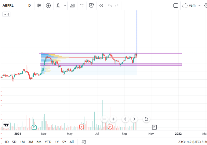
ABFRL
However, when volume is considered in the analysis, the picture becomes clearer. Take note of how volume activity increased during this choppy period. Choppy price action combined with an increase in volume is a sign of distribution when following a trend. When eager buyers entered the market, sellers were eager to take profits and sell their shares. The increased supply kept prices in check, preventing any further price increases. The overhead supply in area above highlighted proved too much for the market to bear, resulting in sharp selling. A trend reversal was clearly taking shape at that point, but we needed one more piece of evidence before making that call.
Tips for Traders
Advantages and disadvantages Volume can be analysed separately and is useful for the following purposes:
• Displaying changes in volume patterns, indicating potential trend changes
• Recognizing price-volume disparities
One disadvantage of using Upside/Downside Volume indicators is that they are only useful for short-term trading decisions and are not suitable for intermediate- or long-term trading decisions. Many useful oscillators and ratios are created by combining up and down volume, and analysing them separately can provide a slightly different perspective on trend strength. The following section expands on this concept.
Volume Oscillator (Upside/Downside)
When examined separately, Upside Volume and Downside Volume can be useful analysis tools, but combining these pieces of data into an oscillator creates a versatile technical tool that can be used for overbought/oversold conditions, showing divergences, and providing positive or negative market signals on zero-line crossovers.
Formulation
This oscillator’s computation is very simple:
Today’s advancing volume – today’s declining volume
Except that the daily results are not added to a running total, this computation is identical to the cumulative volume. This results in a volatile data stream that can be used to identify short-term overbought or oversold conditions.
Divergences in Volume Oscillator (Upside/Downside)
When examined separately, Upside Volume and Downside Volume can be useful analysis tools; however, combining these pieces of data into an oscillator creates a versatile technical tool that can be used in a variety of situations.
In the Upside/Downside Volume Oscillator also displays divergences, which can alert traders to potential trend corrections. The Nifty Stocks may exhibit positive divergence if the price continues to fall while the oscillator makes a series of higher lows. Buyers are more active than sellers, indicating latent market strength. After the divergence was resolved, the Nifty gained nearly 20% in less than three months.
Setup of Trade
The following example generates a trade setup and entry by combining the Nifty Upside/ Downside Volume Oscillator’s 20-day moving average with price movements. Normally, when the price was declining, the 20-day moving average of the Nifty Upside/ Downside Volume Oscillator was making higher lows, indicating a positive divergence. Prices remained stable throughout the rest of the day, with a decrease in selling pressure. A downsloping resistance line connecting the high points of the decline could be drawn, which will be part of our trade entry trigger, along with an upward cross through the zero line in the oscillator.
Accumulation/Distribution
The Accumulation/Distribution line combines price momentum and volume to determine whether traders are accumulating (i.e., buying on a net basis) or distributing (i.e., selling on a net basis) shares. Because volume precedes price, this indicator is most effective before turning points. In many cases, volume patterns shift before price changes, indicating a shift in trader sentiment. Volume-based indicators pick up on these shifts in sentiment, implying that a trend change is on the way.
Now, When the innovative market technician Marc Chaikin set out to improve upon the widely used On-Balance Volume indicator, he took the Accumulation/Distribution line a step further (OBV). Unlike OBV, which accumulated volume based on the relationship between one day’s closing price and the next, Chaikin wanted to quantify the close in terms of whether the period’s action was positive or negative. In order to determine whether the period’s action was positive or negative, his methodology compared the close to the midpoint of the range.
Formulation
The Accumulation/Distribution line is actually computed in two parts.
First, the formula finds the close location value, or CLV:
CLV = [(close – low) – (high – close)] / (high – low)
The CLV can have a maximum value of 1 if the price closes at its highest point for the period, and a minimum value of 1 if the price closes at its lowest point for the period. Any close above the period’s midpoint will have a value greater than zero, while any close below the period’s midpoint will have a value less than zero. The value will be zero if the price closes at the exact midpoint of the period.
Following that, the formula computes the period’s Accumulation/Distribution (A/D) value as follows:
A/D line = yesterday’s A/D value + (CLV * period volume)
Tips for Traders
Accumulation/Distribution is a trend-following indicator. It is useful for the following purposes:
• Confirming trending situations by demonstrating that price and volume are in sync.
• Alerting traders to potential trend changes when the price trend and the indicator diverge.
• Demonstrating whether buyers or sellers are in control by displaying the general flow of money into or out of a security and monitoring whether volume is increasing as the trend moves higher on increased buying pressure or lower on increased selling pressure.
Some disadvantages of using Accumulation/Distribution are as follows:
• The Accumulation/Distribution indicator does not take into account gaps.
• The indicator does not consider the relationship of closing prices from one period to the next because it focuses on the closing price in relation to its own range for the period. For example, if price gaps higher but closes poorly within its range, the indicator will give a negative reading for that period.
• Because price is the most important value in calculating Accumulation/Distribution, good price closes on tepid volume may not show a slowing trend as clearly as poor price closes in the period’s range. As a result, detecting smaller changes in the trend is more difficult.
Normalized volume
Normalized volume is just a method of displaying volume in a uniform scale from security to security or sector to sector. If your trading technique necessitates a certain level of volume to make a deal, and you’re comparing securities, this will allow you to compare apples to apples. John Bollinger, a seasoned technician, recommended this strategy. A common normalisation of trade volume is examined in this article. Normalization makes it easy to compare issues that are on the same relative scale and compare volume totals to their own average. Multiply today’s volume by the moving average of volume values required for your trading, then multiply by 100.
Formulation
This is the formula for normalizing volume: (Replace n with the moving average length of your choice.)
NV = (today’s volume / n period moving average of volume) * 100
Summary
Here, we have covered various different approaches to Volume analysis when combined with Price can give excellent interpretation of the market sentiment and find better probability trades.